
Building a Production-Ready Image Embedding Pipeline
This is the story of building a production-ready image embedding system that processes 11.34 images per second, with a 99.97% success rate, using NVIDIA’s nv-embed-v1 model and Qdrant vector database.

When I set out to process 44,000+ images into vector embeddings, I thought I had it figured out. Download image, call API, store vector. Simple, right?
Spoiler alert: Processing images sequentially at that scale would have taken approximately 30 hours. The final pipeline? Just over an hour.
This is the story of building a production-ready image embedding system that processes 11.34 images per second, with a 99.97% success rate, using NVIDIA’s nv-embed-v1 model and Qdrant vector database.
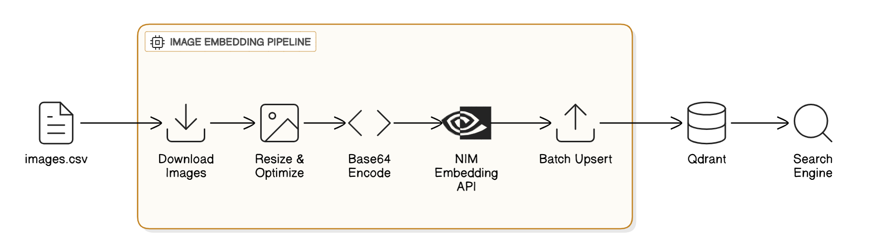
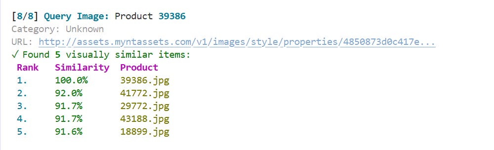
A high-performance, production-ready pipeline for processing fashion product images and generating multimodal embeddings using **NVIDIA NIM APIs**. This system enables semantic image search, visual similarity detection, and cross-modal retrieval (text-to-image and image-to-image search).
The Challenge: Scale Meets Reality
Image embeddings are the foundation of modern visual search systems. Whether you’re building reverse image search, visual recommendation engines, or content moderation systems, you need to convert images into high-dimensional vectors that capture semantic meaning.
The naive approach looks something like this:
for image in images:
    download(image)
    embedding = get_embedding(image)
    store(embedding)
But at scale, this sequential approach becomes a bottleneck nightmare. Each image requires:
Network I/O for downloading (~500ms-2s)
API calls for embedding generation (~1-3s)
Database writes (~100-500ms)
The math is brutal: 44,000 images × 3 seconds average = 36+ hours of processing time.
The Architecture: Orchestrating Chaos
The key insight was recognizing that image processing has two distinct computational bottlenecks with different characteristics:
1. Download-Bound Operations (I/O intensive)
Downloading images from URLs
Network latency and bandwidth constraints
Can be heavily parallelized
2. Embedding-Bound Operations (API rate limits)
NVIDIA API calls for embedding generation
Rate-limited by API quotas
Requires careful throttling
The solution? Dual-semaphore concurrency control.
download_semaphore = asyncio.Semaphore(10)  # 10 concurrent downloads
embedding_semaphore = asyncio.Semaphore(5)   # 5 concurrent API calls
This architecture allows us to:
Download 10 images simultaneously while
Generating embeddings for 5 images in parallel
All while maintaining batched uploads to Qdrant
Think of it like a restaurant kitchen: you don’t want all chefs prepping ingredients OR all chefs cooking. You need both happening in orchestrated parallel.
The Technical Deep Dive
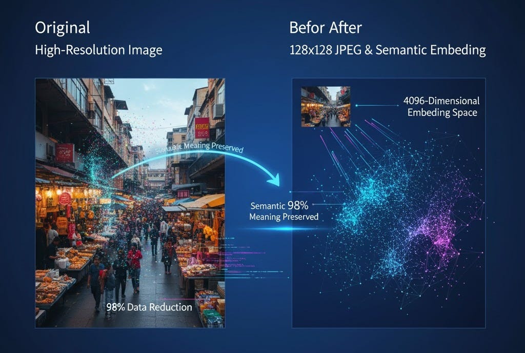
Image Preprocessing: The Token Tax
NVIDIA’s nv-embed-v1 accepts images as base64-encoded data URIs. But there’s a catch: larger images consume more tokens, hitting API limits faster.
The optimization:
image.thumbnail((128, 128), Image.Resampling.LANCZOS)
image.save(buffer, format=”JPEG”, quality=70, optimize=True)
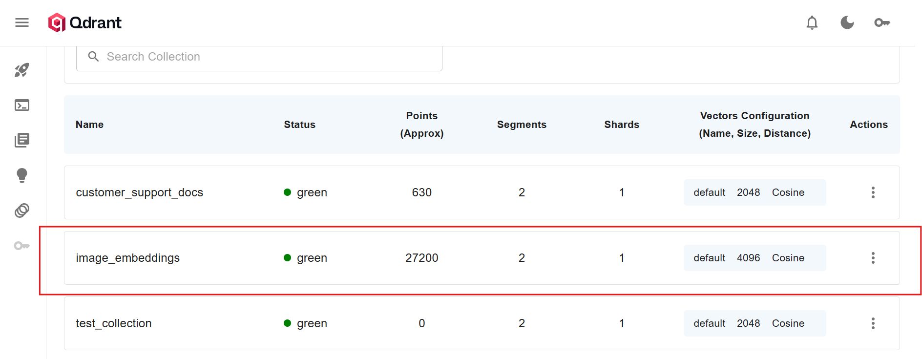
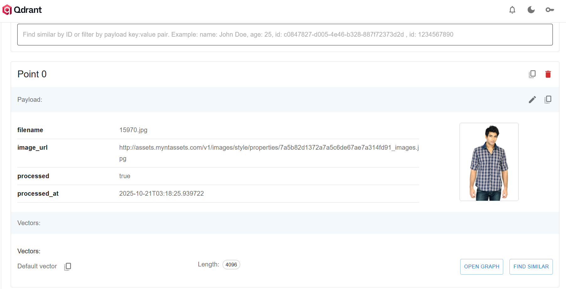
This reduces each image to roughly 8-12KB while maintaining enough visual fidelity for embedding generation. The 4096-dimensional embeddings capture semantic meaning that survives this compression.
Async Everything
The pipeline leverages Python’s asyncio with aiohttp for truly concurrent operations:
connector = aiohttp.TCPConnector(limit=100, limit_per_host=30)
async with aiohttp.ClientSession(connector=connector) as session:
    tasks = [process_image(session, img) for img in images]
    results = await asyncio.gather(*tasks)
Connection pooling prevents socket exhaustion while maximizing throughput.
Batch Uploads: The Hidden Multiplier
Instead of writing each embedding individually to Qdrant, the pipeline batches uploads:
if len(points_buffer) >= 25:
    client.upsert(collection_name=COLLECTION_NAME, points=points_buffer)
    points_buffer = []
Why 25? Testing showed this batch size optimizes the tradeoff between memory usage and network round-trips. Larger batches (50+) showed diminishing returns due to serialization overhead.
The Results: When Architecture Meets Reality
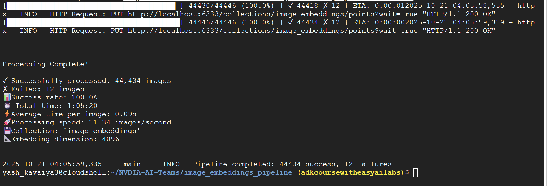
Looking at the terminal output from the production run:
✓ Successfully processed: 44,434 images
✗ Failed: 12 images
📊 Success rate: 99.97%
⏱️  Total time: 1:05:20
⚡ Average time per image: 0.09s
🚀 Processing speed: 11.34 images/second
What this means in practice:
126× faster than sequential processing
Sub-100ms average latency per image
Near-perfect reliability (only 12 failures out of 44k+)
Production-ready scalability
The 12 failures? Dead links, malformed images, timeout errors. Exactly what you’d expect at scale. The pipeline handles them gracefully without stopping the entire process.
Key Learnings: Beyond the Code
1. Semaphores Are Your Friend
Don’t just throw threads at the problem. Separate concerns with independent concurrency limits for different bottleneck types.
2. Fail Fast, Log Everything
Each failure is logged but doesn’t block progress. In production, some images will be inaccessible. Design for partial failures.
3. Configuration Over Hardcoding
Environment variables for API keys, concurrency limits, batch sizes. What works for 10k images might not work for 1M.
4. Monitor The Right Metrics
Images/second (throughput)
Success rate (reliability)
Average latency (user experience)
ETA updates (operational visibility)
5. The Progress Bar Matters
A real-time progress bar with ETA isn’t just nice to have. When processing takes over an hour, stakeholders need visibility. The psychological difference between “running...” and “running... 45% complete, ETA: 32 minutes” is massive.
The Production Architecture
The final system organizes into clean, testable components:
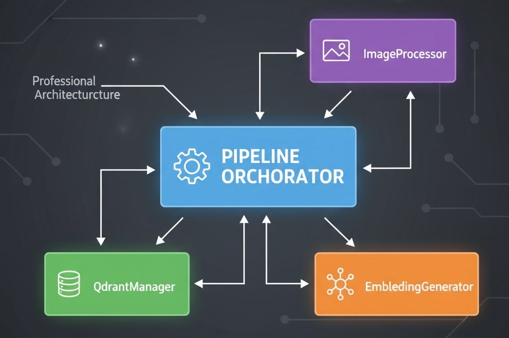
Each component has a single responsibility, making it easy to:
Swap embedding providers (NVIDIA → OpenAI → custom)
Change vector databases (Embeddings → Qdrant)
Add monitoring, retries, or quality checks
Unit test independently
Forward-Looking: What’s Next?
This pipeline processes 44k images in an hour, but the architecture scales further:
Immediate optimizations:
Adaptive concurrency based on API rate limit headers
Smart retries with exponential backoff
Duplicate detection before processing
Streaming mode for real-time ingestion
Architectural evolution:
Distributed processing with message queues (RabbitMQ/Kafka)
GPU-accelerated local embeddings for even faster processing
Multi-region deployment for global image sources
Cost optimization by batching API calls more efficiently
The Bottom Line
Building scalable ML infrastructure isn’t about throwing more compute at the problem. It’s about understanding bottlenecks, orchestrating concurrency intelligently, and designing systems that fail gracefully.
The difference between “it works” and “it works at scale” is often 100× in performance and infinite in production reliability.
Want to build your own image embedding pipeline? The complete code is structured as a production-ready Python package with configuration management, proper logging, and clean abstractions. Start with the basics, measure everything, and optimize the bottlenecks that matter.
Because in production ML, performance isn’t a feature—it’s a requirement.
The final pipeline achieved 11.34 images/second with 99.97% reliability, processing 44,446 images in 1 hour 5 minutes. All embeddings are stored in Qdrant with full metadata for downstream visual search applications.
Tech Stack: Python 3.11+, aiohttp, NVIDIA nv-embed-v1, Qdrant, asyncio